GAUSS sbreak Example

Introduction

This example follows the empirical estimation of Bai and Perron (2003). It uses the GAUSS procedure sbreak to estimate structural breaks in the mean of the US expost real interest rate.

Step 1: Load data

new;
cls;
library tsmt;

// Create file name with full path
fname = getGAUSSHome() $+ "pkgs/tsmt/examples/real_intrate.csv";

// Load all observations from the dataset
y = csvReadM(fname);

// Specify regressors
// Time varying coefficients in z
z = ones(rows(y), 1);

// No time invariant regressors
x = 0;

Step 2: Apply estimation settings

An sbControl control structure is used to control the model characteristics, such as:

• The number of regressors which can change.
• The number of changes to be tested.
• Data trimming.
• Graph and printed output controls.

// Declare sbControl structure
// and fill with default settings
struct sbControl sbc0;
sbc0 = sbControlCreate();

// Number of regressors subject to change
sbc0.q = 1;

// Number of structural changes
sbc0.m = 4;

// Trimming percentage
sbc0.trim = 0.15;

// Minimum length of segment (h > p + q)
sbc0.h = 0;

// Print iteration output
sbc0.printOutput = 1;

// Maximum number of iterations
sbc0.maxIters = 40;

// Turn on graphing capability
sbc0.graphOn = 1;

// Start Date
sbc0.dtstart = dtdate(1961, 01, 01, 0, 00, 00);

// Annual frequency of data
sbc0.frequency = 4;

Step 3: Estimate the model

All output from the sbreak function can be stored in an sbOut output structure.

//Declare output structure
struct sbOut out;

//Estimate model
out = sbreak(y,z,x,sbc0);

Step 4: Output

The printed output from sbreak reads

Global optimization of structural change model
The model with       1.0000000 breaks has SSR :        644.99552
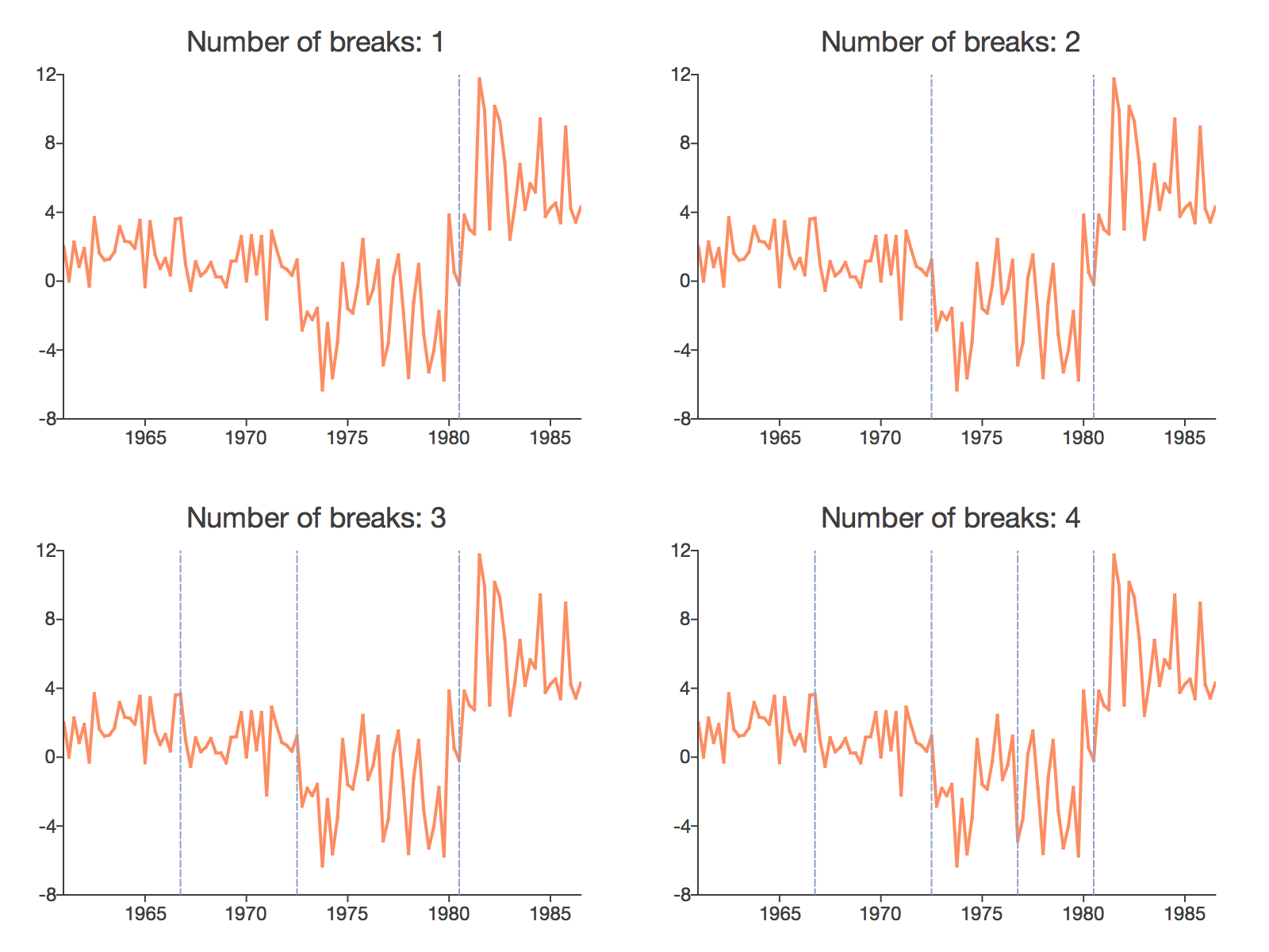
The dates of the breaks are:  Q4-1980
The model with       2.0000000 breaks has SSR :        455.95018
The dates of the breaks are:

         Q4-1972
         Q4-1980
The model with       3.0000000 breaks has SSR :        445.18186
The dates of the breaks are:

         Q1-1967
         Q4-1972
         Q4-1980
The model with       4.0000000 breaks has SSR :        444.87975
The dates of the breaks are:

         Q1-1967
         Q4-1972
         Q1-1977
         Q4-1980  

In addition, the procedure produces graph shown at the top of this page.